Knapsack problem is widely encountered in the real-worlds. When I was a freshman employee in the e-commerce company, this was the first technical problem that our team solved.
In the online advertisement or during the sales promotion, the business operator decides to give the app user coupons of different values to maximize different sales goal, such as profits, Gross Merchandise Value (GMVs), new users and so on. In the meantime, the business operator is constrained by several factors, such as budgets, promotion duration, coupon’s value limits and so on. According to the business description, there are several ways to build a model to help operators to accomplish the sales goal. Some typical models can be established on basis of a 0/1 knapsack problem, a Markov decision process problem or even a reinforcement learning problem. These models are not castel-in-the-air, but can be applicale in the real situations. In Fig.1, I introduce the system design for user promotion recommendation system in Alibaba. This post will majorly focus on the user defined function (UDF) module part. I will discuss it from the point of simulation studies, therefore the feasibility of the algorithm. In the following description, I will introduce a Lagrangian relaxation method to solve a multidimensional knapsack problem1.
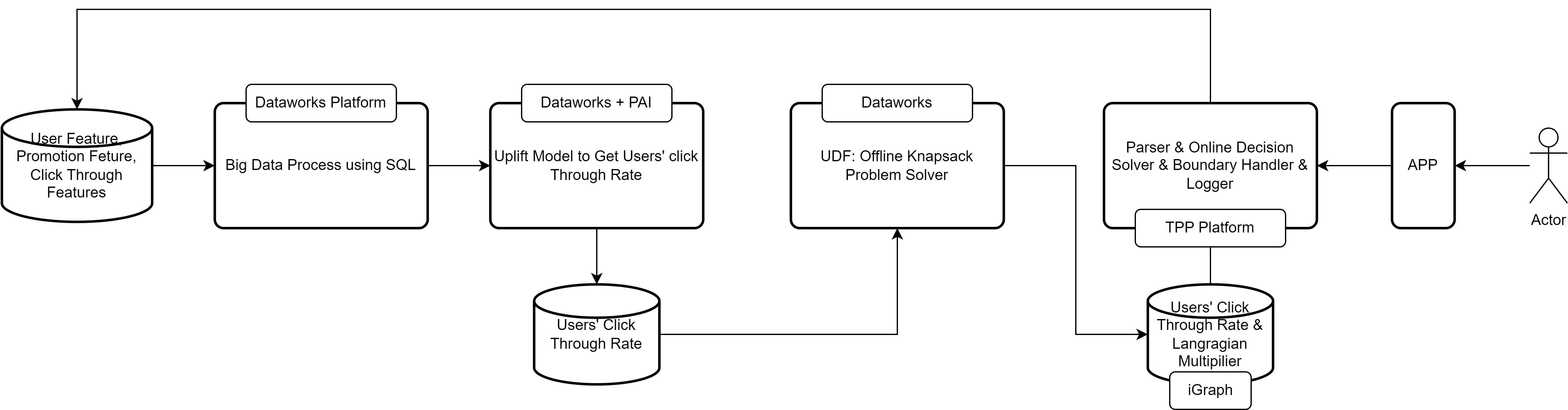 Fig. 1 System Design for User Promotion Recommendation
1. Primal-Dual Formulation
1.1 Formalism
The mathematical description of the multidimesional knapsack problem is as follows,
\[\max \sum_{i=1}^N \sum_{j=1}^{M} p_{ij}x_{ij} \\ \sum_{i=1}^N \sum_{j=1}^M b_{ijk}x_{ij} \le B_k, \quad \forall k \in [K] \\ \sum_{j=1}^M x_{ij} = 1, \quad \forall i \in [N] \\ x_{ij} \in \{0, 1\}, \quad \forall i \in [N], \forall j \in [M]. \tag{1}\]It is a typical description for an operational research problem. We also call it the primal problem. The format might seem intimidating at first glance. Let me explain the mathematical symbols by starting with the subscripts. The subscript $i$ means the index of participants in the promotion. $N$ is the total participants. The subscript $j$ is the index of the coupon’s value. We have $M$ kinds of coupons. $p_{ij}$ describes the sensitivy or probability that the $i$th user’s willing to participate in the promotion given the $j$th coupon’s value. This information can obtained from machine learning of user’s profiles, shopping behavior and price sensitivity. $x_{ij}$ is the decision variables that needs to be figured out in the optimization process. In our scenario, $x_{ij}$ can only take on the value 0 or 1. The goal is to maximize the estimates of total participancy in the promotion campaign given the constraints.
A typical constraint is the budget. In some cases, the operator also cares about the efficiency of the promotion campaign, for example, return of investment (ROI). In generalization, the constraint can be summarized as follows,
\[\sum_{i=1}^N \sum_{j=1}^M b_{ijk}x_{ij} \le B_k, \quad \forall k \in [K], \tag{2}\]where $b_{ijk}$ is the expense of decision $x_{ij}$ for the $k$th constraint. For budget type constraint, if the coupon has a face value $b_j$ and total budget for the campaign is $\tilde{B}N$, the budget constraint can be written as
\[\sum_{i=1}^N \sum_{j=1}^M b_j p_{ij} x_{ij} \le \tilde{B} N . \tag{3}\]For the ROI constraint,
\[\frac{\sum_{i=1}^N \sum_{j=1}^M a_{ij}p_{ij}x_{ij} }{ \sum_{i=1}^N \sum_{j=1}^M b_j p_{ij} x_{ij} } \ge \text{ROI} \quad \forall k \in [K], \tag{4}\]the numerator is the estimated revenue from the campaign and the denominator is the estimated expense of the promotion. $a_{ij}$ is the predicted price of the item that the customer might purchase given the coupon.
Without loss of generality, we provide a Lagrangian relaxation scheme to solve the Equation (1). Every primal problem has a dual problem. To get the dual, We can define the Lagrangian as follows,
\[{\cal L}(x_{ij}, \lambda_k) = \sum_{i=1}^N \sum_{j=1}^M \Big[ p_{ij} - \sum_{k=1}^K \lambda_k b_{ijk} \Big] x_{ij} + \sum_{k=1}^K \lambda_k B_k, \tag{5}\]where $\lambda_k$ is the Lagrangian multipiliers. The dual problem is
\[\min_{\lambda_k} \max_{x_{ij}} {\cal L} (x_{ij}, \lambda_k), \\ \sum_{j=1}^M x_{ij} = 1, \quad \forall k \in [K] \\ \lambda_k \ge 0 \quad k \in [M]. \\ x_{ij} \in \{0, 1\}, \quad \forall i \in [N], \forall j \in [M]. \tag{6}\]In typical primal-dual formulation, the equality constraint will be incorporated in the Lagrangian. In this case, we will use the equaility constraint to establish the explicit relation between $x_{ij}$ and $\lambda_k$. This is very unique in this problem. Otherwise, one has to use $\frac{\partial {\cal L}}{\partial x_{ij}} = 0$ to get the relation between decision variables and Lagrangian multipilers, for example in the algrithm of support vector machine. To elaborate this, Let us take $\lambda_k$ fixed.
For a fixed set of Lagrangian multipliers $\lambda_k^*$, we will have the following problem,
\[\max_{x_{ij}} \sum_{i=1}^N \sum_{j=1}^M \Big[ p_{ij} - \sum_{k=1}^K \lambda_k^* b_{ijk} \Big] x_{ij} + \sum_{k=1}^K \lambda_k^* B_k, \\ \sum_{j=1}^M x_{ij} = 1, \quad \forall k \in [K]. \\ x_{ij} \in \{0, 1\} \quad \forall i \in [N] \quad \forall j \in [M]. \tag{7}\]Now, the problem can be splited into sub-problems, such that
\[\max_{x_{ij}} \sum_{i=1}^N \sum_{j=1}^M \Big[ p_{ij} - \sum_{k=1}^K \lambda_k^* b_{ijk} \Big] x_{ij} \Longleftrightarrow \sum_{i=1}^N \max_{x_{ij}} \sum_{j=1}^M \Big[ p_{ij} - \sum_{k=1}^K \lambda_k^* b_{ijk}. \Big] x_{ij} \tag{8}\]Here we neglect the constant part $\sum_{k=1}^K \lambda_k^* B_k$. The maximization of the overall revenue constrained by resource limits becomes the maximization of every customer’s expense subjected to resource limits. The optimal solution of the decision variables for every customer is,
\[x_{ij} = 1, \quad j = \arg \max_{j} p_{ij} - \sum_{k=1}^K \lambda_k^* b_{ijk}, \\ \text{otherwise} \quad x_{ij} = 0. \tag{9}\]Equation.(9) is the so-called relation between decision variables and Lagrangian multipliers, $x_{ij}(\lambda)$. This allows us to use it in the following minimization procedures,
\[\min_{\lambda_k} {\cal L} (\lambda_k) \\ \text{s.t.} \quad \lambda_k \ge 0, \forall k \in [K] \tag{10}\]We can solve it by a gradient descent method or a stochastic descent method. It is noticed that $x_{ij}(\lambda)$ has singularities. This singularity is ignored by only providing the gradient of ${\cal L}$ with respect $\lambda_r$,
\[\frac{\partial {\cal L}}{\partial \lambda_r} = -\lambda_r \sum_i^N \sum_j^M b_{ijr} x_{ij} + \lambda_r B_r. \tag{11}\]In the following case, we used an Adam optimizer to find the approximate optimal solution2. In order to evaluate the solution, python-MIP package which applies Coin-or branch and cut algorithm is used to get the ground truth optimal value to evalute the gap. The optimality is defined as,
\[\text{Optimality} = 1 - \frac{Q - Q^*}{Q^*}. \tag{12}\]where $Q^*$ is the objective value of optimal solution from an exact algorithm. $Q$ is the objective value of the solution. Moreover, as the dual descent method doesn’t guarantee the constraints, we utilize the following metric to evaluate the constraint satisfaction ratio,
\[\text{SAT} = \sum_{k=1}^K \frac{\max(\sum_i^N \sum_j^N b_{ijk}x_{ij} - B_k,0)}{\| B_k \| } \tag{13}\]2.2 Online Inference
In an online application, customers are served sequentially. Give the critical time constraints, with response times limited to a few milliseconds. The click-through probability $p_{ij}$ predicted by the machine learning model can be used by the inference engine to determine the optimal coupon for each customer by using Equation.(9).
2. Simulated Case Study
2.1 Online Flow Control
In online advertising, a web owner has $M$ advertisements to distribute. To maximize the total click-through rate, the problem can be formulated as follows,
\[\max \sum_{i=1}^N \sum_{j=1}^{M} p_{ij}x_{ij} \\ \sum_{i=1}^N x_{ij} \le (s_j + \epsilon) N, \quad \forall j \in [M] \\ \sum_{j=1}^M x_{ij} = 1, \quad \forall i \in [N] \\ \sum_{j=1}^M s_j = 1 \\ x_{ij} \in \{0, 1\}, \quad \forall i \in [N], \forall j \in [M]. \tag{11}\]where $s_j$ represents the ratio of impressions for the $j$th ads, $p_{ij}$ is the estimated click-throught rate of the $j$th ads for the $i$th user, and $\epsilon$ is the minimal relaxation parameter to guarantee a feasible solution for an exact algorithm. The Lagrangian of Equation.(1) is,
\[{\cal L}(\lambda_j, x_{ij}) = \sum_{i=1}^N \sum_{j=1}^M \Big[ p_{ij} - \lambda_j \Big] x_{ij} + \sum_{j=1}^M \lambda_j s_j N, \tag{12}\]and its derivative is,
\[\frac{\partial {\cal L}}{\partial \lambda_r} = -\sum_i x_{ir} + s_r N. \tag{13}\]2.2 Simulated Results
To assess feasibility of the primal-dual approximation method, we conducted simulations across several cases, measuring both optimality and constraint satisfaction. In the following simulation, we fixed the minimal relaxation parameter $\epsilon$ to $0.01$ and empolyed an equal convergence criterion for the ADAM algorithm iterations. Figure 1 demonstrates that all simulated cases achieved objective values close to those obtained using the Python-MIP solver.
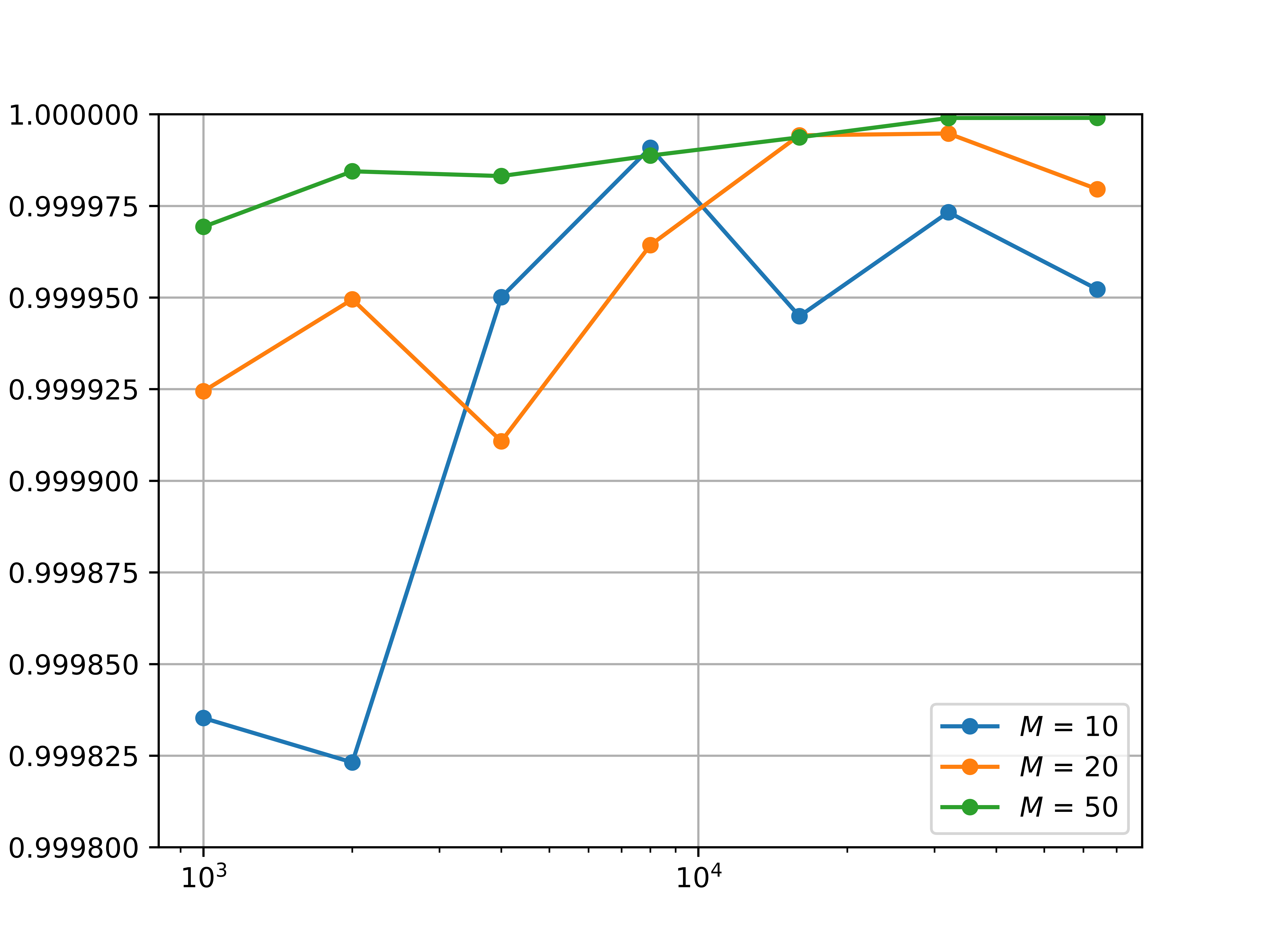 Fig. 2 Optimality for different cases
While the primal-dual approximation method often struggles to achieve perfect constraint satisfaction, it remains a viable approach for scenarios involving soft constraints. Conversely, for cases where strict adherence to inequality constraints is critical, this method may not be suitable.
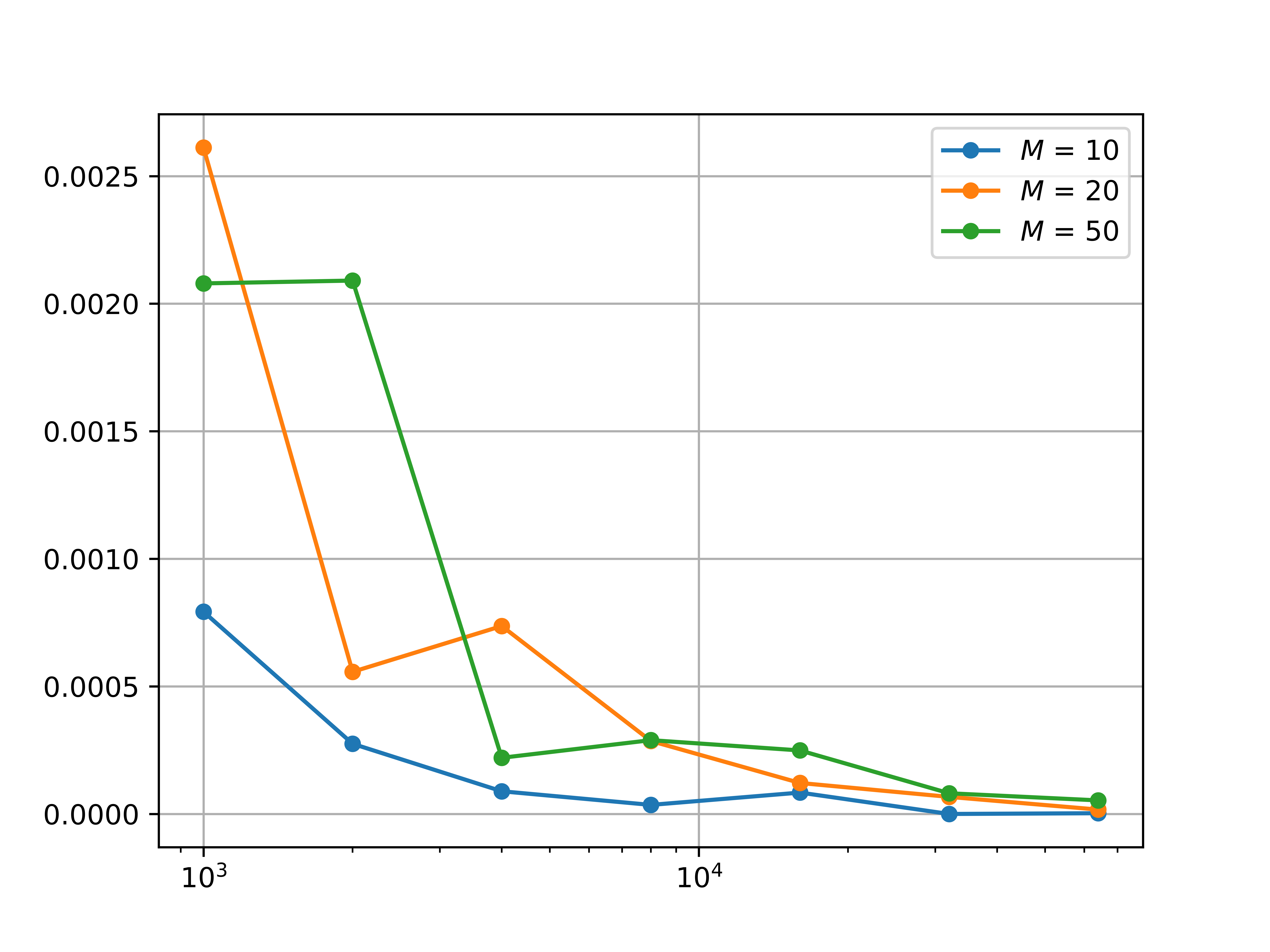 Fig. 3 Constraint satisfaction
2.3 Code
We provide the code below,
import os
import time
import numpy as np

import bottleneck as bn
import math
import random

import mip
import logging

def linear_fun(x, x1, y1, x2, y2):
    """
    linear function (x1, y1) and (x2, y2)
    """
    slope = (y2 - y1) / (x2 - x1)

    return slope * (x - x1) + y1

def log_fun(x, x1, y1, x2, y2):
    """
    logarithmic function (x1, y1) and (x2, y2)
    """
    a = (y2 - y1) / (math.log(x2) - math.log(x1))
    b = y1 - a * math.log(x1)

    return a * np.log(x) + b

def mono_fun(x, x1, y1, x2, y2):
    """
    construct a monotonoically increaseing function
    between (x1, y1) and (x2, y2)
    """
    funs = {
        "linear_fun": linear_fun,
        "log_fun": log_fun
    }

    rnd_name = random.choice(list(funs.keys()))
    rnd_fun = funs[rnd_name]

    return rnd_fun(x, x1, y1, x2, y2)

def noiser(x, n, std_dev):
    """
    Add the noise to the function.
    """
    return x + np.random.normal(0.0, std_dev, n)

class TrafficPara(object):
    """
    Online Traffic Model: parameters builder
    """
    def __init__(self, N, M, eps, seed = 1337) -> None:
        np.random.seed(seed)
        self._N = N
        self._M = M
        self._eps = eps
        self._pij = np.random.rand(N, M)
        self._sj = np.random.randint(0, N, M)
        self._sj = self._sj/np.sum(self._sj) + eps

    @property
    def N(self):
        return self._N

    @property
    def M(self):
        return self._M

    @property
    def eps(self):
        return self._eps

    @property
    def pij(self):
        return self._pij

    @property
    def sj(self):
        return self._sj


class TrafficDual(object):
    """
    """
    def __init__(self, para : TrafficPara, filename='app.log', level = logging.INFO) -> None:
        self.N = para.N
        self.M = para.M
        self.pij = para.pij
        self.sj = para.sj
        self.lamb = np.random.rand(self.M)

        self.logger = logging.getLogger(filename)
        self.logger.setLevel(level)
        ch = logging.StreamHandler()
        ch.setLevel(level)
        formatter = logging.Formatter('%(asctime)s - %(name)s - %(levelname)s - %(message)s')
        ch.setFormatter(formatter)
        self.logger.addHandler(ch)

    def func(self, lamb):
        """Lagrangian function
        """
        varphi = self.pij - lamb
        # partition, Partition array so that the
        # first 3 elements (indices 0, 1, 2) are the
        # smallest 3 elements (note, as in this example,
        # that the smallest 3 elements may not be sorted):
        varphi = -bn.partition(-varphi, 1, -1)[:, 0]
        return np.sum(varphi) * self.N * np.sum(lamb * self.sj)

    def dfunc(self, lamb):
        """derivative of Lagrangian
        """
        x = np.zeros((self.N, self.M))
        varphi = self.pij - lamb
        varphi_idx = bn.argpartition(-varphi, 1, -1)
        for i in range(self.N):
            for j in range(1):
                x[i, varphi_idx[i, j]] = 1
        return -np.sum(x, axis=0) + self.sj * self.N

    @property
    def x(self):
        x = np.zeros((self.N, self.M))
        varphi = self.pij - self.lamb
        varphi_idx = bn.argpartition(-varphi, 1, -1)
        for i in range(self.N):
            for j in range(1):
                x[i, varphi_idx[i,j]] = 1
        return x

    @property
    def objective_value(self):
        x = np.zeros((self.N, self.M))
        varphi = self.pij - self.lamb
        varphi_idx = bn.argpartition(-varphi, 1, -1)
        for i in range(self.N):
            for j in range(1):
                x[i, varphi_idx[i,j]] = 1
        return np.sum(self.pij * x)

    def checkConstraint(self):
        """check the violation the major constraint"""
        return np.sum(self.x, axis=0) - self.sj * self.N

    def checkAbsConstraint(self):
        """check the magnitude of violation of the constraints"""
        val = np.sum(self.x, axis=0) - self.sj * self.N
        return np.sum(val[val > 0])/self.N

    def optimize(self, optimizer_name = "adam", tolx=1e-5, tolf=1e-5, nitermax = 10000):

        optimizers = {
            "adam": self.adam
        }
        optimizer = optimizers[optimizer_name]
        self.lamb = optimizer(tolx, tolf, nitermax)

    def adam(self, tolx=1e-4, tolf=1e-4, nitermax = 10000):
        """
        Adam algorithm to find the optimal value
        """
        self.logger.info(f"Iteration Begins!")

        theta0 = self.lamb

        start = time.time()

        alpha, beta1, beta2, eps = 0.001, 0.9, 0.999, 1e-8
        beta1powert, beta2powert = 1.0, 1.0

        niter = 0

        theta_old = theta0
        ndim = len(theta0)
        mold = np.zeros(ndim)
        vold = np.zeros(ndim)

        fold = self.func(theta0)

        while niter < nitermax:

            self.logger.debug(f"Iteration: {niter}")
            niter += 1

            g = self.dfunc(theta_old)
            mnew = beta1 * mold + (1-beta1)*g
            vnew = beta2 * vold + (1-beta2)*g*g

            beta1powert *= beta1
            beta2powert *= beta2

            mhat = mnew/(1 - beta1powert)
            vhat = vnew/(1 - beta2powert)

            theta_new = theta_old - alpha * mhat / (np.sqrt(vhat) + eps)

            self.logger.debug(f"theta_old: {theta_old}")
            self.logger.debug(f"theta_new: {theta_new}")

            theta_new[theta_new<0.0] = 0.0

            if np.sqrt(np.inner(theta_new - theta_old, theta_new - theta_old)) < tolx:

                end = time.time()
                self.logger.info(f"Exit from gradient")
                self.logger.info(f"Running time: {end - start}")
                return theta_new

            self.logger.debug(f"fold: {fold}")
            fnew = self.func(theta_new)
            self.logger.debug(f"fnew: {fnew}")

            if np.abs(fold - fnew) < tolf:
                end = time.time()
                self.logger.info(f"Exit from function")
                self.logger.info(f"Running time: {end - start}")
                return theta_new

            theta_old = theta_new
            fold = fnew
            mold = mnew
            vold = vnew

            self.logger.debug(f"{niter}th iteration \t theta: {theta_old} \
                obj func: {theta_new} \t grad: {g}")

        self.logger.warning("EXCEED THE MAXIMUM ITERATION NUMBERS!")
        end = time.time()
        self.logger.warning(f"Running time : {end - start}")

        return theta_new


class TrafficMIP(object):
    """MIP solver
    """
    def __init__(self, para : TrafficPara, filename='mip.log', level = logging.INFO,
    maxseconds=300) -> None:
        self.N = para.N
        self.M = para.M
        self.pij = para.pij
        self.sj = para.sj

        self.maxseconds = maxseconds

        self.logger = logging.getLogger(filename)
        self.logger.setLevel(level)
        ch = logging.StreamHandler()
        ch.setLevel(level)
        formatter = logging.Formatter('%(asctime)s - %(name)s - %(levelname)s - %(message)s')
        ch.setFormatter(formatter)
        self.logger.addHandler(ch)

        I = range(self.N)
        V = range(self.M)

        self.model = mip.Model()

        self.x = [[self.model.add_var(var_type = mip.BINARY) for j in V] for i in I]

        self.model.objective = mip.maximize(mip.xsum(self.pij[i][j] * self.x[i][j] for i in I for j in V))

        # local constraints, only 3 benefits recommended for
        for i in I:
            self.model += mip.xsum(self.x[i][j] for j in V) == 1

        # global constraints, the coupons are limited by numbers
        for j in V:
            self.model += mip.xsum(self.x[i][j] for i in I) <= self.sj[j] * self.N

        self.model.optimize(max_seconds=maxseconds)

    def checkAbsConstraint(self):
        """check the magnitude of violation of the constraints
        """
        val = []
        for j in range(self.M):
            sumval = 0
            for i in range(self.N):
                sumval += self.x[i][j].x
            val.append(sumval)
        val = np.array(val)
        val -= self.sj * self.N
        return np.sum(val[val > 0])/self.N


def optimality(q, qs):
    return 1 - np.abs(q - qs)/qs


if __name__ == "__main__":

    para = TrafficPara(1000, 10, 0.01, 13)
    model_dual = TrafficDual(para)
    model_dual.optimize()
    print(model_dual.checkAbsConstraint())

    model_mip  = TrafficMIP(para, maxseconds=30)
    print(model_mip.checkAbsConstraint())

    q  = model_dual.objective_value
    qs = model_mip.model.objective_value

    print(optimality(q, qs))
Conclusion
A primal-dual approximate method is provided to solve the multidimensional knapsack problem. A case study is provided with codes.