We review the electromagnetic field theory of circular waveguide, particular about the TE and TM mode. Most part of the discussion comes from David M. Pozar’s book.
Electromagnetic Field Theory
The Figure shows the geometry of a hollow, round metal pipe with inner radius $a$. Such a waveguide supports TE and TM waveguide modes. We use cylindrical coordinate system to address the formalism of the electromagnetic field inside the waveguide1.
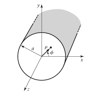 Fig.1 Geometry of circular waveguide.
Assuming that the waveguide is source free, we can write Maxwell’s equation as
\[\begin{gathered} \nabla \times \mathbf{E} = - j \omega \mu \mathbf{H}, \\ \nabla \times \mathbf{H} = j \omega \epsilon \mathbf{E} \end{gathered} \tag{1}\]In the cylindrical coordinate system, we can write the electric and magnetic ansatz of field as
\[\begin{gathered} \mathbf{E}(\rho, \phi, z) = [\hat{\rho}E_{\rho}(\rho, \phi) + \hat{\phi}E_{\phi}(\rho, \phi) + \hat{z}E_{z}(\rho, \phi)] e^{-j \beta z}, \\ \mathbf{H}(\rho, \phi, z) = [\hat{\rho}H_{\rho}(\rho, \phi) + \hat{\phi}H_{\phi}(\rho, \phi) + \hat{z}H_{z}(\rho, \phi)] e^{-j \beta z}, \end{gathered} \tag{2}\]where $E_{\rho}(\rho, \phi)$, $E_{\phi}(\rho, \phi)$, $H_{\rho}(\rho, \phi)$ and $H_{\phi}(\rho, \phi)$ represent the transverse electric and magnetic filed components in the $\rho-\phi$ plane, and $E_z(\rho, \phi)$ and $H_z(\rho, \phi)$ are the longitudinal electric and magnetic field components. We will expand the Eq.(1) for each component. To do that, we will need the following vector analysis expression in the cylindrical system.
\[\nabla \times \mathbf{A} = \hat{\rho} (\frac{1}{\rho} \frac{\partial A_z}{\partial \phi} - \frac{\partial A_{\phi}}{\partial z} ) + \hat{\phi} (\frac{\partial A_{\rho}}{\partial z} - \frac{\partial A_{z}}{\partial \rho} ) + \hat{z} \frac{1}{\rho} [ \frac{ \partial ( \rho A_{\phi})}{\partial \rho} - \frac{\partial A_{\rho}}{\partial \phi} ]. \tag{3}\]With that, we can rewrite Eq.(1) for each component as
\[\begin{gathered} \frac{1}{\rho} \frac{\partial E_z}{\partial \phi} + j \beta E_{\phi}= -j \omega \mu H_{\rho}, \\ -j\beta E_{\rho} - \frac{\partial E_z}{\partial \rho} = -j \omega \mu H_{\phi}, \\ \frac{1}{\rho}E_{\phi} - \frac{1}{\rho} \frac{\partial E_{\rho}}{\partial \phi} = -j \omega \mu H_z, \\ \frac{1}{\rho} \frac{\partial H_z}{\partial \phi} + j \beta H_{\phi}= j \omega \epsilon E_{\rho}, \\ -j\beta H_{\rho} - \frac{\partial H_z}{\partial \rho} = j \omega \epsilon E_{\phi}, \\ \frac{1}{\rho}H_{\phi} - \frac{1}{\rho} \frac{\partial H_{\rho}}{\partial \phi} = j \omega \epsilon E_z, \end{gathered} \tag{4}\]The four transverse component can be expressed in terms of longitudinal component $E_z$ and $H_z$,
\[\begin{gathered} E_{\rho} = -\frac{j}{k_c^2} (\beta \frac{\partial E_z}{\partial \rho} + \frac{\omega \mu}{\rho} \frac{\partial H_z}{\partial \phi}), \\ E_{\phi} = -\frac{j}{k_c^2} (\frac{\beta}{\rho} \frac{\partial E_z}{\partial \phi} - \omega \mu \frac{\partial H_z}{\partial \rho}), \\ H_{\rho} = \frac{j}{k_c^2} (\frac{\omega \epsilon}{\rho} \frac{\partial E_z}{\partial \phi} - \beta \frac{\partial H_z}{\partial \rho}), \\ H_{\phi} = -\frac{j}{k_c^2} (\omega \epsilon \frac{\partial E_z}{\partial \rho} + \frac{\beta}{\rho} \frac{\partial H_z}{\partial \phi}), \end{gathered} \tag{5}\]where $k_c^2 = k^2 - \beta^2$. The waveguide can both support TE ($E_z = 0$) and TM ($H_z = 0$) modes.
TE modes
For transverse electric (TE) mode, the field component are given by
\[\begin{gathered} E_{\rho} = -\frac{j\omega \mu}{k_c^2}\frac{1}{\rho} \frac{\partial H_z}{\partial \phi}, \\ E_{\phi} = \frac{j \omega \mu }{k_c^2} \frac{\partial H_z}{\partial \rho}, \\ H_{\rho} = -\frac{j \beta }{k_c^2} \frac{\partial H_z}{\partial \rho}, \\ H_{\phi} = -\frac{j \beta}{k_c^2} \frac{1}{\rho} \frac{\partial H_z}{\partial \phi}. \end{gathered} \tag{6}\]The longitudinal component $H_z$ is a solution to the wave equation
\[\nabla^2 H_z + k^2 H_z = 0. \tag{7}\]If, the above equation can be expressed in cylindrical coordinates as
\[\Big( \frac{\partial^2}{\partial \rho^2} + \frac{1}{\rho} \frac{\partial}{\partial \rho} + \frac{1}{\rho^2}\frac{\partial^2}{\partial \phi^2} + k_c^2 \Big) H_z(\rho, \phi) = 0. \tag{8}\]We can apply the method of separation of variables to let
\[H_z(\rho, \phi) = R(\rho) P(\phi), \tag{9}\]and substitute into Eq. (8) to obtain
\[\frac{\rho^2}{R} \frac{d^2 R}{d \rho^2} + \frac{\rho}{R}\frac{d R}{d \rho} + \rho^2 k_c^2 = \frac{-1}{P} \frac{d^2 P}{d \phi^2}. \tag{10}\]The left side of the equation depends only on $\rho$, while the right side depends only on $\phi$. Thus, each side must be equal to a constant, which we will call $k_{\phi}^2$. Then, we have
\[\frac{d^2 P}{d \phi^2} + k_{\phi}^2 P = 0. \tag{11}\]In addition,
\[\rho^2\frac{d^2 R}{d \rho^2} + \rho\frac{d R}{d \rho} + (\rho^2 k_c^2 - k_{\phi}^2 )R = 0. \tag{12}\]The general solution to Eq.(11) is
\[P(\phi) = A \sin (k_{\phi} \phi) + B \cos (k_{\phi} \phi). \tag{13}\]In order to satisfy the periodicity of $H_z$ in $\phi$ direction, i.e., $H_z(\rho, \phi) = H_z (\rho, \phi \pm 2m \pi)$, $k_{\phi}$ must be an integer, $n$. Thus, Eq.(13) becomes
\[P(\phi) = A \sin (n \phi) + B \cos (n \phi). \tag{14}\]and Eq.(12) becomes
\[\rho^2\frac{d^2 R}{d \rho^2} + \rho\frac{d R}{d \rho} + (\rho^2 k_c^2 -n^2 )R = 0, \tag{15}\]which is Bessel’s differential equation2. The solution is
\[R(\rho) = C J_n (k_c \rho) + D N_n(k_c \rho), \tag{16}\]where $J_n(x)$ and $N_n(x)$ are the Bessel’s functions of first and second kinds, respectively. In order to have a sensible idea of Bessel’s functions, we can plot its first $n$th order. The computation of the Bessel’s functions or other special function are also addressed in another Prof. Jianmin Jin’s and his collaborator’s book3.
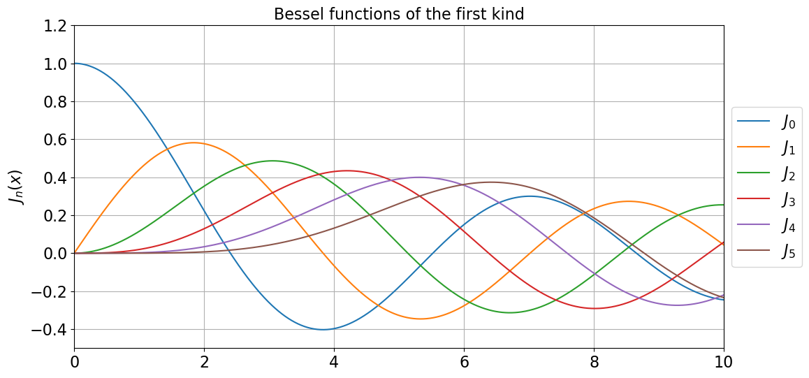 Fig.2 Bessel functions
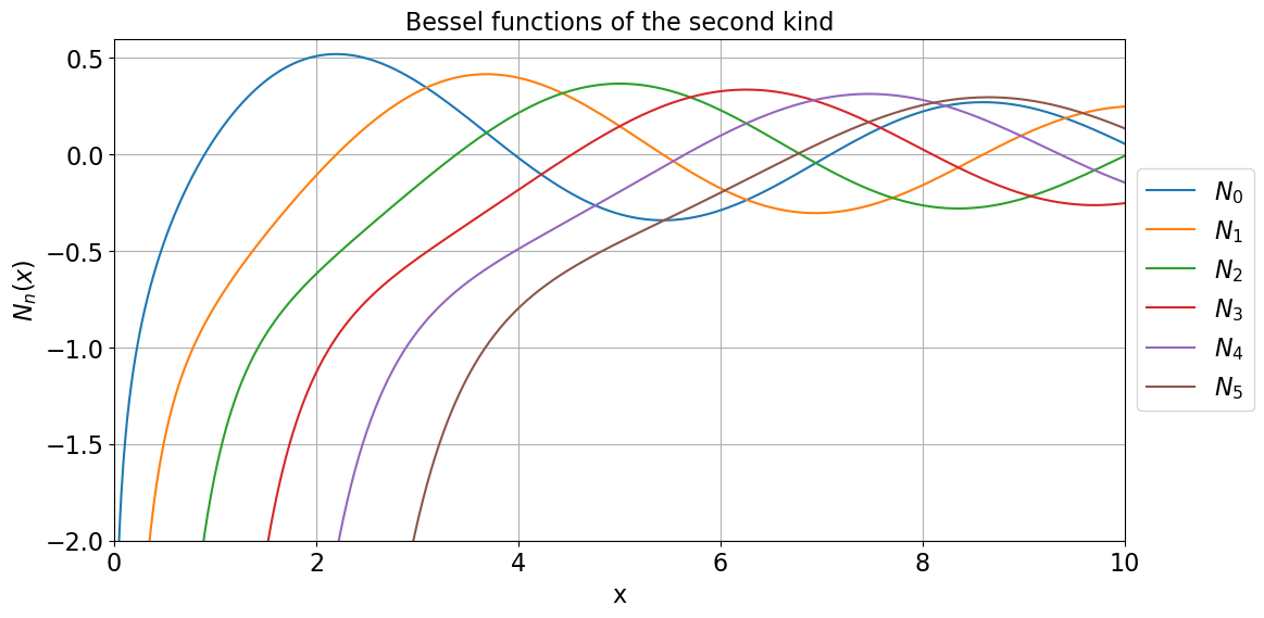 Fig.3 Bessel functions of second kind
Because Bessel’s functions of second kind (Neumann functions) $N_n(x)$ is infinite at $\rho=0$, this term is physically unacceptable for a circular waveguide, thus $D=0$. The solution for $H_z$ can then be simplified to
\[H_z(\rho, \phi) = (A \sin (n \phi) + B \cos (n \phi)J_n(k_c \rho). \tag{17}\]We now impose the boundary condition $E_{tan} = 0$ on the waveguide’s wall. Because $E_z = 0$, we must have that
\[E_{\phi}(\rho, \phi) = 0 \quad \text{at} \quad \rho = a. \tag{18}\]From Eq. (6), we find $E_{\phi}$ from $H_z$ as
\[E_{\phi}(\rho, \phi, z) = \frac{j \omega \mu}{k_c} (A \sin n\phi + B \cos n\phi) J'_n(k_c \rho) e^{-j\beta z}, \tag{19}\]where $J’_n(k_c \rho)$ is the derivative of $J_n$. In order to satisfy the boundary condition, we must have
\[J'_n(k_c a) = 0. \tag{20}\]We denote the root of as $\chi’_{nm}$, so that $J’_n(\chi’_{nm}) = 0$, where $\chi’_{nm}$ is the $m$th root of $J’_n$. Then $k_c$ must have the value
\[k_{cnm} = \frac{\chi'_{nm}}{a}. \tag{21}\]Several zeroes $\chi’_{nm}$ of the derivative of the first kind Bessel function $J’_n(x)$ are listed below.
| m = 1 | m = 2 | m = 3 | m = 4 | M = 5 | |
|---|---|---|---|---|---|
| n = 0 | 3.832 | 7.016 | 10.173 | 13.324 | 16.471 |
| n = 1 | 1.841 | 5.331 | 8.536 | 11.706 | 14.864 |
| n = 2 | 3.054 | 6.706 | 9.969 | 13.17 | 16.348 |
| n = 3 | 4.201 | 8.015 | 11.346 | 14.586 | 17.789 |
| n = 4 | 5.318 | 9.282 | 12.682 | 15.964 | 19.196 |
The $\text{TE}_{nm}$ modes are defined by the cutoff wave number $k_{cnm} = \chi’_{nm}/a$. The propagation constant of the $\text{TE}_{nm}$ mode is
\[\beta_{nm} = \sqrt{k^2 - k_c^2} = \sqrt{k^2 - (\frac{\chi'_{nm}}{a})^2}, \tag{22}\]with a cutoff frequency of
\[f_{cnm} = \frac{k_c}{2 \pi \sqrt{\mu \epsilon}} = \frac{\chi'_{nm}}{2 \pi a \sqrt{\mu \epsilon}}. \tag{23}\]The first TE mode to propagate is the mode with the smallest $\chi’_{nm}$, which from the above table is seen to be $\text{TE}_{11}$ mode. The next smallest TE mode is $\text{TE}_{21}$ mode, and then $\text{TE}_{01}$ mode, and so on.
Finally, we summarize the transverse field components
\[\begin{gathered} E_{\rho} = \frac{- j \omega \mu n}{k_c^2 \rho} (A \cos n\phi - B \sin n\phi) J_n(k_c \rho) e^{-j\beta z}, \\ E_{\phi} = \frac{j \omega \mu}{k_c} (A \sin n\phi + B \cos n\phi) J'_n(k_c \rho) e^{-j\beta z}, \\ H_{\rho} = \frac{- j \beta}{k_c} (A \sin n\phi + B \cos n\phi) J'_n(k_c \rho) e^{-j\beta z}, \\ H_{\phi} = \frac{- j \beta n}{k_c^2 \rho} (A \cos n\phi - B \sin n\phi) J_n(k_c \rho) e^{-j\beta z}. \end{gathered} \tag{24}\]There are still two remaining constants $A$ and $B$. The actual amplitude will depend on the excitation of the waveguide.
TM modes
For transverse magnetic (TM) mode, the field component are given by
\[\begin{gathered} E_{\rho} = -\frac{j \beta}{k_c^2} \frac{\partial E_z}{\partial \rho}, \\ E_{\phi} = -\frac{j \beta}{k_c^2} \frac{1}{\rho} \frac{\partial E_z}{\partial \phi} , \\ H_{\rho} = \frac{j \omega \epsilon}{k_c^2} \frac{1}{\rho} \frac{\partial E_z}{\partial \phi}, \\ H_{\phi} = -\frac{j \omega \epsilon}{k_c^2} \frac{\partial E_z}{\partial \rho} , \end{gathered} \tag{25}\]Similarly, for the TM modes of the circular waveguide, we solve for $E_z$ from the wave equation in cylindrical coordinates,
\[\Big( \frac{\partial^2}{\partial \rho^2} + \frac{1}{\rho} \frac{\partial}{\partial \rho} + \frac{1}{\rho^2}\frac{\partial^2}{\partial \phi^2} + k_c^2 \Big) E_z = 0, \tag{26}\]where $E_z (\rho, \phi, z) = E_z (\rho, \phi)e^{-j \beta z}$. We will have the solution
\[E_z(\rho, \phi) = (A \sin n\phi +B \cos n\phi) J_n (k_c \rho). \tag{27}\]If we directly impose the boundary condition
\[E_{\phi}(\rho, \phi) = E_z(\rho, \phi) = 0 \quad \text{at} \quad \rho = a, \tag{28}\]we must have
\[J_n (k_c a)= 0, \tag{29}\]or
\[k_c = \chi_{nm} / a, \tag{30}\]where $\chi_{nm}$ is the $m$th root of $J_n(x)$, that is, $J_n(\chi_{nm}) = 0$. Table shows the several zeros of Bessel’s function,
| m = 1 | m = 2 | m = 3 | m = 4 | M = 5 | |
|---|---|---|---|---|---|
| n = 0 | 2.405 | 5.520 | 8.654 | 11.792 | 14.931 |
| n = 1 | 3.832 | 7.016 | 10.173 | 13.324 | 16.471 |
| n = 2 | 5.136 | 8.417 | 11.620 | 14.796 | 17.960 |
| n = 3 | 6.38 | 9.761 | 13.015 | 16.223 | 19.409 |
| n = 4 | 7.588 | 11.065 | 14.373 | 17.616 | 20.827 |
The $\text{TM}_{nm}$ modes are defined by the cutoff wave number $k_{cnm} = \chi_{nm}/a$. The propagation constant of the $\text{TM}_{nm}$ mode is
\[\beta_{nm} = \sqrt{k^2 - k_c^2} = \sqrt{k^2 - (\frac{\chi_{nm}}{a})^2}, \tag{31}\]with a cutoff frequency of
\[f_{cnm} = \frac{k_c}{2 \pi \sqrt{\mu \epsilon}} = \frac{\chi_{nm}}{2 \pi a \sqrt{\mu \epsilon}}. \tag{32}\]The first TM mode to propagate is the mode with the smallest $\chi_{nm}$, which from the above table is seen to be $\text{TM}_{01}$ mode.
The transverse fields can be summarized as,
\[\begin{gathered} E_{\rho} = \frac{-j \beta}{k_c} (A \sin n\phi + B \cos n\phi) J'_n(k_c \rho) e^{-j\beta z}, \\ E_{\phi} = \frac{- j \beta n}{k_c^2 \rho} (A \cos n\phi - B \sin n\phi) J_n(k_c \rho) e^{-j\beta z}, \\ H_{\rho} = \frac{ j \omega \epsilon n}{k_c^2 \rho} (A \cos n\phi - B \sin n\phi) J_n(k_c \rho) e^{-j\beta z}, \\ H_{\phi} = \frac{- j \omega \epsilon}{k_c} (A \sin n\phi + B \cos n\phi) J'_n(k_c \rho) e^{-j\beta z}. \end{gathered} \tag{33}\]Electric and Magnetic Mode Plots
Figure 4 shows some electric and magnetic fields line for the first 24 TE and TM modes in the circular waveguide4.
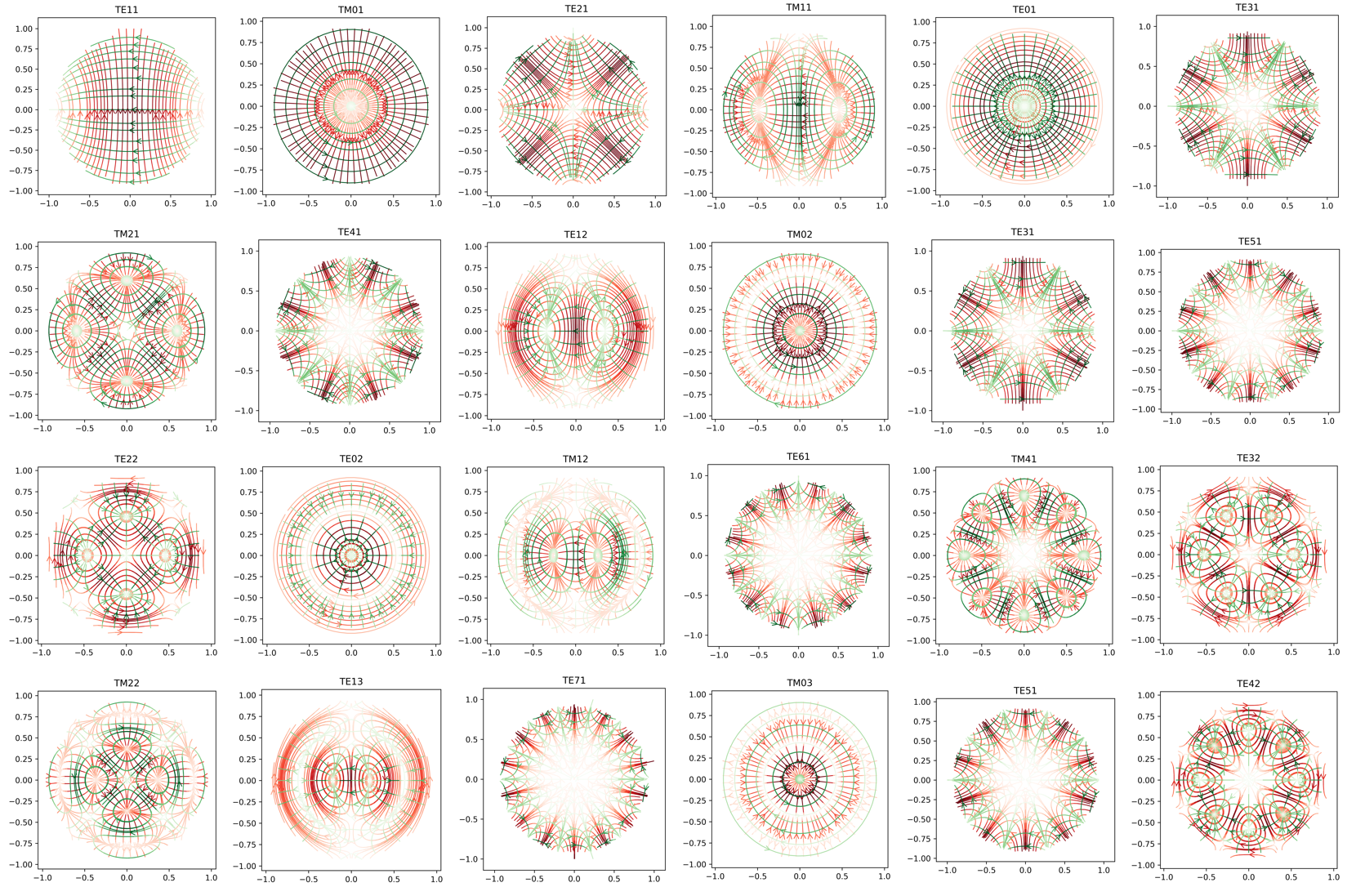 Fig.4 TE and TM mode of the first 24 modes in a circular waveguide. The red streamlines are electric field lines and the green streamlines are magnetic field lines.
Codes
import numpy as np
import matplotlib.pyplot as plt

from scipy.special import jv, yv, jvp
import scipy.special as special

def compute_TE_real(rho, phi, kc, n):
    """
    Computes the TE modes of a circular waveguide.
    As the E and H are in the same phase, we can use the imaginary part.
    """
    E_rho = - n / (kc*kc * rho) * ( - np.sin(n * phi)) * jv(n, kc * rho)
    E_phi =   1.0 / kc * (  np.cos(n * phi))   * jvp(n, kc * rho)
    H_rho = - 1.0 / kc * (  np.cos(n * phi)) * jvp(n, kc * rho)
    H_phi = - 1.0 * n / (kc*kc * rho) * ( - np.sin(n * phi)) * jv(n, kc * rho)

    return E_rho, E_phi, H_rho, H_phi

def compute_TM_real(rho, phi, kc, n):
    """
    Computes the TM modes of a circular waveguide.
    As the E and H are in the same phase, we can use the imaginary part.
    """
    E_rho = - 1.0 / kc * ( np.cos(n * phi)) * jvp(n, kc * rho)
    E_phi = - n / (kc*kc * rho) * ( - np.sin(n * phi)) * jv(n, kc * rho)
    H_rho =  1.0 * n / (kc*kc * rho) * (- np.sin(n * phi)) * jv(n, kc * rho)
    H_phi = - 1.0 / kc * ( np.cos(n * phi)) * jvp(n, kc * rho)

    return E_rho, E_phi, H_rho, H_phi


def plotField(MODE, n, m):
    """
    Plots the field of the TE or TM mode.
    """
    x = np.linspace(-1.0, 1.0, 100)
    y = np.linspace(-1.0, 1.0, 100)
    X, Y = np.meshgrid(x, y)

    radii = np.sqrt(X**2 + Y**2)
    theta = np.arctan2(Y, X)


    if MODE == "TE":
        # For TE modes, first find out the cutoff wave number kcnm
        kcnm = special.jnp_zeros(n, 5)[m-1] / 1.0
        E_rho, E_phi, H_rho, H_phi = compute_TE_real(radii, theta, kcnm, n)
    elif MODE == "TM":
        # For TM modes, first find out the cutoff wave number kcnm
        kcnm = special.jn_zeros(n, 5)[m-1] / 1.0
        E_rho, E_phi, H_rho, H_phi = compute_TM_real(radii, theta, kcnm, n)

    E_rho[radii > 0.95 ] = np.nan
    E_phi[radii > 0.95 ] = np.nan
    H_rho[radii > 0.95 ] = np.nan
    H_phi[radii > 0.95 ] = np.nan

    Ex = (E_rho * np.cos(theta) - E_phi * np.sin(theta))
    Ey = (E_rho * np.sin(theta) + E_phi * np.cos(theta))

    E_norm = np.sqrt(np.abs(Ex)**2 + np.abs(Ey)**2)

    Hx = (H_rho * np.cos(theta) - H_phi * np.sin(theta))
    Hy = (H_rho * np.sin(theta) + H_phi * np.cos(theta))

    H_norm = np.sqrt(np.abs(Hx)**2 + np.abs(Hy)**2)

    fig, ax = plt.subplots(figsize=(4, 4))
    ax.set_aspect('equal')

    # Enforce the margins, and enlarge them to give room for the vectors.
    ax.use_sticky_edges = False
    ax.margins(0.07)

    ax.streamplot(X, Y, Ex, Ey, density = 0.8, color=E_norm, cmap = "Reds",arrowstyle='->',
                arrowsize=1.5, linewidth=1, broken_streamlines=False)
    ax.streamplot(X, Y, Hx, Hy, density = 0.5, color=H_norm, cmap = "Greens" ,arrowstyle='->',
                arrowsize=1.5, linewidth=1, broken_streamlines=False)


    ax.set_title('{}{}{}'.format(MODE, n, m))
    plt.tight_layout()
    plt.savefig('{}_{}{}.png'.format(MODE, n, m), dpi=600)
    plt.close()


if __name__ == "__main__":

    #
    plotField("TE", 7, 1)
Reference
-
Pozar, David M. Microwave engineering: theory and techniques. John wiley & sons, 2021. ↩
-
Arfken, George B., and Hans J. Weber. Mathematical Methods for Physicists. Academic Press, 2005. ↩
-
Zhang, Shanjie and Jin, Jianming. “Computation of Special Functions”, John Wiley and Sons, 1996, Chapter 5. ↩
-
Aline Tomasian. “How to Use Circular Ports in the RF Module”. Comsol Blog. [https://www.comsol.com/blogs/how-to-use-circular-ports-in-the-rf-module#References] ↩