This post is about mathematical formulas for my reference.

Integration by parts

For ordinary functions of one variable, the rule for integration by parts follows immediately from integrating the product rule

$$\begin{align*} \frac{d}{dx}(fg) &= \frac{df}{dx}g + f\frac{dg}{dx}, \\ \int_a^b \frac{d}{dx} (fg) \, dx &= \int_a^b \frac{df}{dx}g \, dx + \int_a^b f \frac{dg}{dx} \, dx, \\ fg |_a^b &= \int_a^b \frac{df}{dx}g \, dx + \int_a^b f \frac{dg}{dx} \, dx. \end{align*}$$

Rearraging, we obtain

$$\int_a^b \frac{df}{dx}g \, dx = fg |_a^b - \int_a^b f \frac{dg}{dx} \, dx.$$

In an analogous way, we can obtain a rule for integration by parts for the divergence of a vector field by starting from the product rule for the divergence

$$\nabla \cdot (f \mathbf{G}) = (\nabla f) \cdot \mathbf{G} + f (\nabla \cdot \mathbf{G}).$$

integrating both sides yields

$$\int \nabla \cdot (f \mathbf{G}) \, d\tau = \int (\nabla f) \cdot \mathbf{G} \, d\tau + \int f (\nabla \cdot \mathbf{G}) \, d\tau .$$

Now use the divergence theorem to rewrite the first term, leading to

$$\int (f \mathbf{G}) \cdot \, d\mathbf{A} = \int (\nabla f) \cdot \mathbf{G} \, d\tau + \int f (\nabla \cdot \mathbf{G}) \, d\tau .$$

which can be rearranged to

$$\int f (\nabla \cdot \mathbf{G}) \, d\tau = \int (f \mathbf{G}) \cdot \, d\mathbf{A} - \int (\nabla f) \cdot \mathbf{G} \, d\tau .$$

which is the desired integration by parts.

Typical Steps in Finite Element Analysis of Electromagnetics

We have the divergence theorem,

$$\int_{\Omega} \nabla \cdot \vec{w} \ d\Omega = \int_{\Gamma} \vec{w} \cdot \hat{n} \ d \Gamma, \tag{1}$$

where $\Omega$ is the integral domain, and $\Gamma$ is the integral boundary, and $\vec{w}$ is a vector field, and $\hat{n}$ is the normal to the integral boundary outward.

For a scalar field $u$ in Poisson equation of the electrostatics, we wiil have the following steps used in the formulation of weak form of the Poisson equation.

$$\nabla \cdot (v \ \epsilon \nabla u) = \nabla v \cdot (\epsilon \nabla u) + v \nabla \cdot (\epsilon \nabla u),$$

where $v$ is the test scalar field. If apply integral over domain to the above equation, we have

$$\int_{\Omega} v \nabla \cdot (\epsilon \nabla u) \ d \Omega = \int_{\Omega} \nabla \cdot (v \epsilon \nabla u) \ d \Omega + \int_{\Omega} \nabla v \cdot \epsilon \nabla u \ d \Omega \\ = \int_{\Gamma} v \epsilon \nabla u \cdot \hat{n} \ d\Gamma + \int_{\Omega} \nabla v \cdot \epsilon \nabla u \ d \Omega$$

where we apply the divergence theorem in the second step.

For a vector filed $\vec{u}$ in the Helmholtz equation of waveguide problems, we will have the following steps used in the formulation of weak form of the Helmholtz equation.

Recall from the vector analysis, we have the following equality,

$$\nabla \cdot (\vec{a} \times \vec{b}) = \vec{b} \cdot \nabla \times \vec{a} - \vec{a} \cdot \nabla \times \vec{b}. \tag{2}$$

We have the following steps in the formulation of Helmholtz equation with Eq. (2),

$$\nabla \cdot [ \vec{v} \times (\frac{1}{\mu_r} \nabla \times \vec{u} ) ] = \frac{1}{\mu_r} \nabla \times \vec{u} \cdot \nabla \times \vec{v} - \vec{v} \cdot [ \nabla \times (\frac{1}{\mu_r} \nabla \times \vec{u} ) ],$$

where $\vec{v}$ is the test vector field. We can apply the integral over the domain for the above equation, we have

$$\int_{\Omega} \vec{v} \cdot [ \nabla \times (\frac{1}{\mu_r} \nabla \times \vec{u} ) ] \ d \Omega = \int_{\Omega} \frac{1}{\mu_r} \nabla \times \vec{u} \cdot \nabla \times \vec{v} \ d \Omega - \int_{\Omega} \nabla \cdot [ \vec{v} \times (\frac{1}{\mu_r} \nabla \times \vec{u} ) ] \ d \Omega, \\ = \int_{\Omega} \frac{1}{\mu_r} \nabla \times \vec{u} \cdot \nabla \times \vec{v} \ d \Omega - \int_{\Gamma} \vec{v} \times (\frac{1}{\mu_r} \nabla \times \vec{u} ) \cdot \hat{n} \ d \Gamma, \\ = \int_{\Omega} \frac{1}{\mu_r} \nabla \times \vec{u} \cdot \nabla \times \vec{v} \ d \Omega - \int_{\Gamma} \frac{1}{\mu_r} \nabla \times \vec{u} \cdot (\hat{n} \times \vec{v}) \ d \Gamma,$$

where we apply divergence theorem for the second step and we apply the following equality for the third step,

$$\vec{a} \cdot (\vec{b} \times \vec{c} ) = \vec{b} \cdot (\vec{c} \times \vec{a}) = \vec{c} \cdot (\vec{a} \times \vec{b} ).$$

Boundary conditions ¹

One-dimensional scalar field $\phi$

For a one-dimensional scalar field $\phi$, we have three kinds of boundary conditions.

• boundary condition of the first kind:

$$\phi = p,$$

which is typically called as Dirichlet boundary condition.

• boundary condition of the third kind:

$$[\alpha \frac{d \phi}{dx} + \gamma \phi] = q,$$

which is called Robin boundary condition.

• boundary condition of the second kind:

$\gamma = 0$, a special case of the third boundary condition, is also termed as Neumann condition.

Two-dimensional scalar field $\phi$

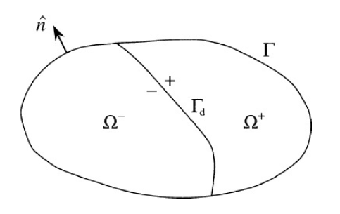Fig. Two-dimensional domain having a discontinuity interface .

For a two-dimensional scalar field $\phi$, the three kinds of boundary conditions are

• boundary condition of the first kind, also known as Dirichlet boundary condition:

$$\phi = p \quad \text{on} \quad \Gamma_1$$

• boundary condition of the third kind, known as Robin boundary:

$$(\alpha_x \frac{\partial \phi}{\partial x} \hat{x} + \alpha_y \frac{\partial \phi}{\partial y} \hat{y})\cdot \hat{n} + \gamma \phi = q \quad \text{on} \quad \Gamma_2$$

• boundary condition of the second kind:

The boundary condition of the second kind is a special case of the above equation with $\gamma=0$ which is known as Neumann boundary condition.

Three-dimensional scalar field $\phi$

For a three-dimensional scalar field $\phi$, the three kinds of boundary conditions are

• boundary condition of the first kind, also known as Dirichlet boundary condition:

$$\phi = p$$

• boundary condition of the third kind, known as Robin boundary:

$$(\alpha_x \frac{\partial \phi}{\partial x} \hat{x} + \alpha_y \frac{\partial \phi}{\partial y} \hat{y} + \alpha_z \frac{\partial \phi}{\partial z}\hat{z} )\cdot \hat{n} + \gamma \phi = q,$$

• boundary condition of the second kind:

The boundary condition of the second kind is a special case of the above equation with $\gamma=0$ which is known as Neumann boundary condition.

Reference