This post is about S-parameter of networks.

1. Impedance of Resistor, Capacitor and Inductor¹

Electrical impedance is the opposition that a circuit presents to a current when a voltage is applied. It is a generalization of resistance from direct current (DC) to alternating current (AC), and, like resistance, it is measured in ohms (Ω). Impedance is the combined effect of resistance, inductance, and capacitance in an AC circuit.

Unlike resistance, which has only magnitude, impedance extends the concept of resistance to alternating current (AC) circuits, and possesses both magnitude and phase. Therefore, the impedance is represented as a complex number. The symbol is usually $Z$. Polar form $| Z | \angle \theta$ is sometimes used to represent impedance. Cartesian complex number representation is more often used. The impedance is defined as

where the real part of the impedance is the resistance $R$ and the imaginary part is the reactance $X$.

1.1 Resistor

The impedance of an ideal resistor is purely real and is called resistive impedance:

where $R$ is the resistance with SI unit of Ohm ($\Omega$).

1.2 Capacitor

The impedance of capacitors is

where $\omega$ is the angular frequency and $C$ is the capacitance with SI unit of Farad ($F$).

1.3 Inductor

The impedance of inductor is

where $L$ is the inductance of SI unit of Henry ($H$).

1.4 Combining impedance

For components connected in series, the current through each circuit element is the same. The total impedance is the sum of the component impedances.

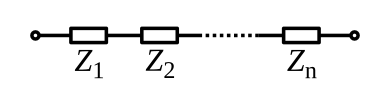Fig.1 Components in series.

For components connected in parallel, the voltage across each circuit element is the same. Hence the inverse total impedance is the sum of the inverses of the component impedances:

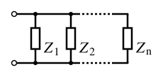Fig.2 Components in parallel.

For two components connected in parallel, the impedance is

2. Impedance and Scattering Matrix²

An arbitrary N-port microwave network is shown in Figure. The incident $(V_n^+, I_n^+)$ and reflected $(V_n^-, I_n^-)$ waves are defined at a specific point on the $n$th plane. The impedance matrix $\mathbf{Z}$ of the microwave network relates the voltages and currents as

where $V_n = V_n^+ +V_n^-$ and $I_n = I_n^+ - I_n^-$.

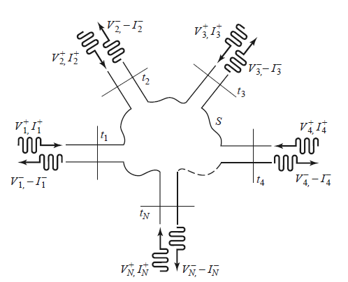Fig.3 Components in parallel.

From the above equation, we see that the matrix element $Z_{ij}$ can be computed as

The formula states that $Z_{ij}$ can be found by driving port $j$ with the current $I_j$, open circuiting all other ports (thus $I_k = 0$ for $k \neq j$), and measuring the open-circuit voltage at port $i$.

The S-parameter (or Scattering matrix) describes how wave interacts with the device under test (DUT)³. For historical reason, the word scatter is used to refer hit or collide. The wave that scatters back to the source is called reflected wave and the wave that scatters through the device is referred to transmitted wave. In the frequency domain, the instrument used to measure the reflected and transmitted response of the sine waves is a vector network analyzer (VNA). Vector refers to the fact that both the magnitude and phase of the sine wave are being measured. A scalar network analyzer just measures the amplitude of the sine wave, not its phase. The frequency domain reflected and transmitted terms are referred to as specific S-parameters, such as S11 and S21 or the return and insertion loss.

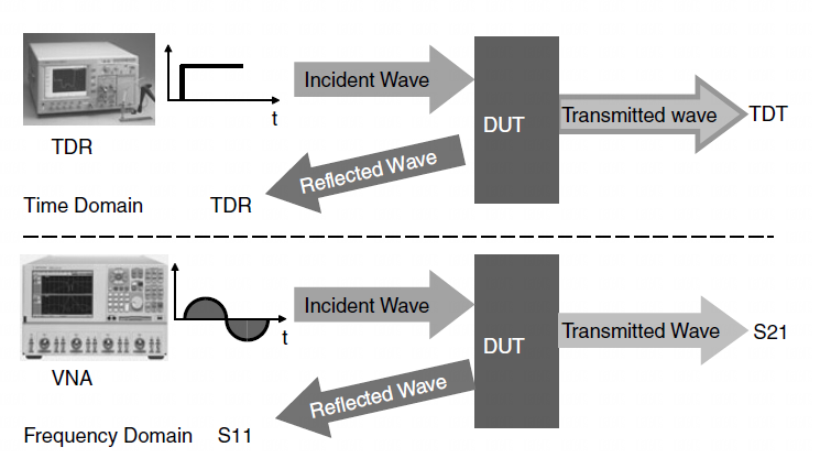Fig.4 Components in parallel.

The scattering matrix is defined in relation to theses incident and reflected voltage waves as

A specific element of the scattering matrix can be determined as

In words, the above equation says $S_{ij}$ is found by driving port $j$ with an incident wave of voltage $V_j^+$ and measuring the reflected wave amplitude $V_i^-$ coming out of port $i$. The incident waves on all ports except the $j$th port are set to zero, which means that all ports should be terminated in matched loads to avoid reflections. Thus, $S_{ii}$ is the reflection coefficient seen looking into port $i$ when all other ports are terminated in matched loads, and $S_{ij}$ is the transmission coefficient from port $j$ to port $i$ when all other ports are terminated in matched loads.

We can derive the scattering matrix from impedance matrix. First, we must assume that the characteristic impedance, $Z_{0n}$ , of all ports are identical. The total voltage and current at the $n$th port can be written as

From the definition of $\mathbf{Z}$ , we can have

The above equation can be organized as

where $\mathbf{I}$ is the identity matrix. Therefore, the scattering matrix can be computed as

3. Two Port Network

3.1 T-Network

We can apply the above theory to a two-port T-network in the Fig.5 of Pozar².

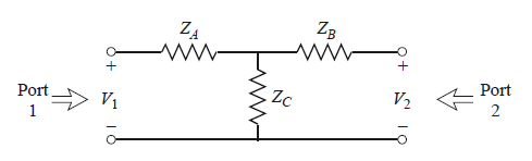Fig.5 T-network.

The $Z_{11}$ can be found as the input impedance of port 1 when port 2 is open-circuited:

Similarly, $Z_{22}$ is $Z_B + Z_C$. The transfer impedance $Z_{12}$ can be found by measuring the open-circuit voltage at port 1 when a current $I_2$ is applied at port 2,

Therefore, the impedance matrix for two-port T-network is

We assume that the matched impedances of port 1 and port 2 are identical, $Z_{01} = Z_{02} $. In matrix form, it gives

The scattering matrix of the T-network can be computed from Eq.(14).

3.2 $\Pi$- Network

We consider a pi-network in the following⁴:

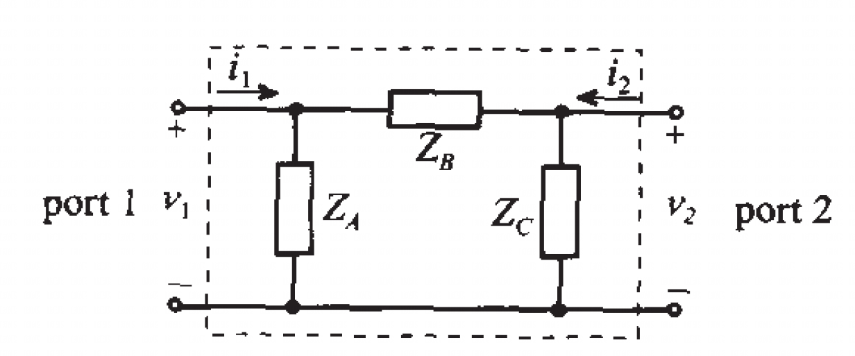Fig.6 pi-network.

The $Z_{11}$ can be found as the input impedance of port 1 when port 2 is open-circuited:

Similarly, we can obtain $Z_{22}$ by driving port 2 when port 1 is open-circuited, $Z_{22} = \frac{Z_C(Z_A + Z_B)}{Z_A + Z_B + Z_C}$.

The value of $Z_{12}$ can be found as the ratio of open circuit voltage drop $V_1$ measured across port 1 to the current $I_2$,

The voltage drop $V_1$ can be computed from voltage divider rule $V_1 = \frac{Z_A}{Z_A + Z_B} V_2$. The voltage $V_2$ can be computed from Ohm’s law as $V_2 = I_2 \Big(Z_C || (Z_A + Z_B)\Big)$. Thus, the transfer impedance element $Z_{12}$ is

Similarly, $Z_{21}$ can be determined in the same way. Thus, the impedance matrix for the $\Pi$ - network is written in the form

3.3 Square Network

We can consider a square network which is named by me. This type of network is often observed in the literature.

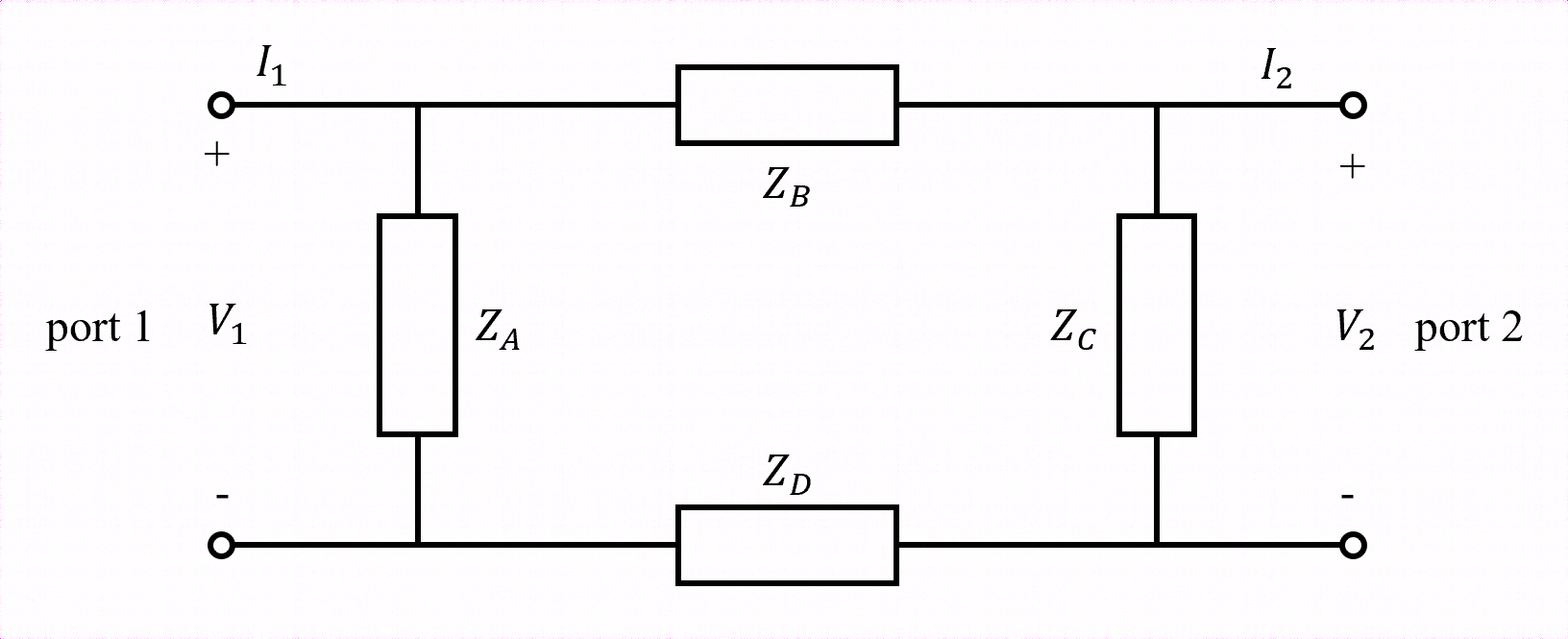Fig.7 Square-network.

The $Z_{11}$ can be found as the input impedance of port 1 when port 2 is open-circuited:

Similarly, we can obtain $Z_{22}$ by driving port 2 when port 1 is open-circuited, $Z_{22} = \frac{Z_C(Z_A + Z_B + Z_D)}{Z_A + Z_B + Z_C + Z_D}$.

The value of $Z_{12}$ can be found as the ratio of open circuit voltage drop $V_1$ measured across port 1 to the current $I_2$,

The voltage drop $V_1$ can be computed from voltage divider rule $V_1 = \frac{Z_A}{Z_A + Z_B +Z_D} V_2$. The voltage $V_2$ can be computed from Ohm’s law as $V_2 = I_2 \Big(Z_C || (Z_A + Z_B + Z_D) \Big)$. Thus, the transfer impedance element $Z_{12}$ is

Similarly, $Z_{21}$ can be determined in the same way.

Thus, the impedance matrix for the $\Pi$ - network is written in the form

4. Application

4.1 Validation of Theory by Qucs Studio

We can use Example 4.4 of Pozar² to do a simple exercise. We can begin with T-network. The following is the realization of the code

import numpy as np
import matplotlib.pyplot as plt

class Network:
    """
    Parent class for all 2*2 network types.
    """
    def __init__(self):
        """
        Initializes the network with default parameters.
        """
        self.Z = np.zeros(shape=(2, 2), dtype=np.complex128)
        self.S = np.zeros(shape=(2, 2), dtype=np.complex128)

    def _constructSMatrix(self, Z0):
        """
        Assume that the matched impedance is identical with the parameter Z0.
        Constructs the S matrix for the network.
        """
        self.Z0 = Z0
        U = np.eye(2) * Z0
        self.S = np.linalg.inv(self.Z + U) @ (self.Z - U)
        
class TNetwork(Network):
    """
    Two-port T-network
    """
    def __init__(self, za, zb, zc, Z0):
        
        super().__init__()
        self.za = za
        self.zb = zb
        self.zc = zc

        self._constructZMatrix()
        self._constructSMatrix(Z0)

    def _constructZMatrix(self):
        """
        Construct the Z matrix of the T-network
        """
        z11 = self.za + self.zc
        z12 = self.zc
        z21 = self.zc
        z22 = self.zb + self.zc

        self.Z = np.array([[z11, z12],
                           [z21, z22]])

tnet = TNetwork(8.56, 8.56, 141.8, 50)

print("Z matrix:")
print(tnet.Z)

print("S matrix:")
print(tnet.S)

print("Insertion loss:")
print(20 * np.log10(np.abs(tnet.S[0, 1])))

Below is the output of the code,

Z matrix:
[[150.36 141.8 ]
 [141.8  150.36]]
S matrix:
[[4.43981086e-05 7.07694671e-01]
 [7.07694671e-01 4.43981086e-05]]
Insertion loss:
-3.003081489040847

This simple codes can be validated by Qucs Studio software. We can build the network as follows,

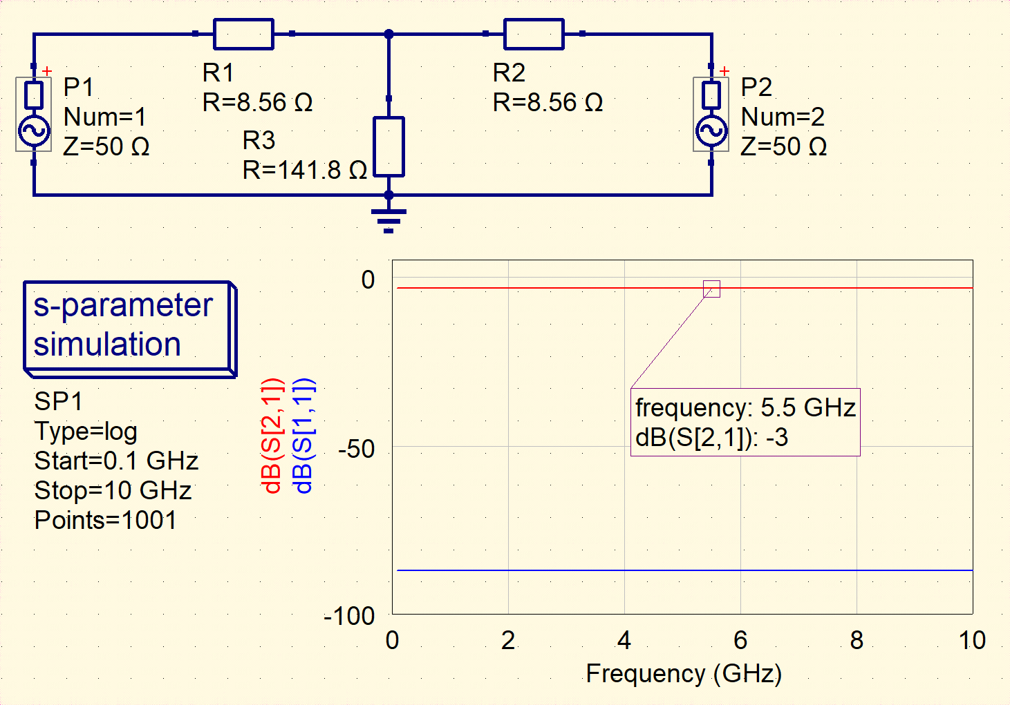Fig.8 Qucs simulation of T-network

Next, we can realize the $\Pi$-network.

class PiNetwork(Network):
    """
    Two-port Pi-network
    """
    def __init__(self, za, zb, zc,  Z0):
        
        super().__init__()
        self.za = za
        self.zb = zb
        self.zc = zc

        self._constructZMatrix()
        self._constructSMatrix(Z0)

    def _constructZMatrix(self):
        """
        Construct the Z matrix of the T-network
        """
        zsum = self.za + self.zb + self.zc
        z11 = self.za * (self.zb + self.zc) / zsum
        z12 = self.za * self.zc / zsum
        z21 = self.za * self.zc / zsum
        z22 = self.zc * (self.za + self.zb) / zsum

        self.Z = np.array([[z11, z12],
                           [z21, z22]])

pinet = PiNetwork(1, 2, 3, 50)

print("Z matrix:")
print(pinet.Z)

print("S matrix:")
print(pinet.S)

print(f"S11: {20 * np.log10(np.abs(pinet.S[0, 0]))}")
print(f"S12: {20 * np.log10(np.abs(pinet.S[0, 1]))}")
print(f"S21: {20 * np.log10(np.abs(pinet.S[1, 0]))}")
print(f"S22: {20 * np.log10(np.abs(pinet.S[1, 1]))}")

This is the output of the above code:

Z matrix:
[[0.83333333 0.5       ]
 [0.5        1.5       ]]
S matrix:
[[-0.96740099  0.01910098]
 [ 0.01910098 -0.94193302]]
S11: -0.2878694209607549
S12: -34.378886767932826
S21: -34.378886767932826
S22: -0.519599575008295

The above code is validated by Qucs Studio.

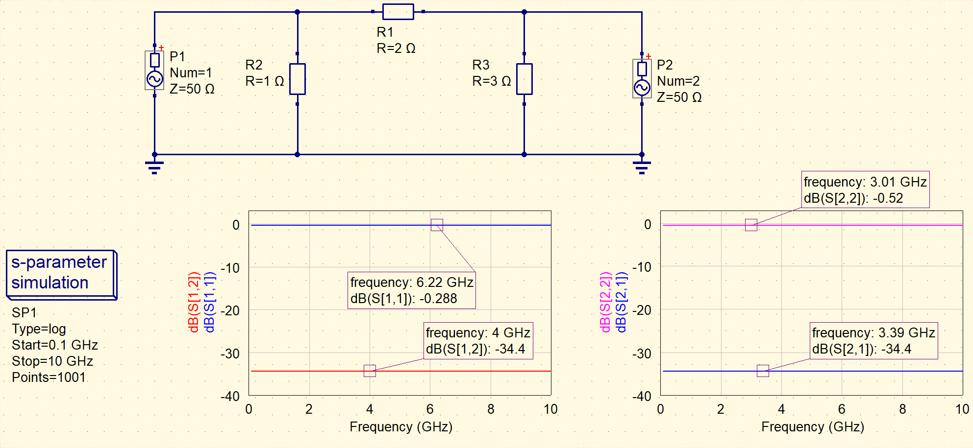Fig.9 Qucs simulation of pi-network

At last, we can realize the square network.

class SquareNetwork(Network):
    """
    Two-port Square-network
    """
    def __init__(self, za, zb, zc, zd, Z0):
        
        super().__init__()
        self.za = za
        self.zb = zb
        self.zc = zc
        self.zd = zd

        self._constructZMatrix()
        self._constructSMatrix(Z0)

    def _constructZMatrix(self):
        """
        Construct the Z matrix of the T-network
        """
        zsum = self.za + self.zb + self.zc + self.zd
        z11 = self.za * (self.zb + self.zc + self.zd) / zsum
        z12 = self.za * self.zc / zsum
        z21 = self.za * self.zc / zsum
        z22 = self.zc * (self.za + self.zb + self.zd) / zsum

        self.Z = np.array([[z11, z12],
                           [z21, z22]])

snet = SquareNetwork(1, 2, 3, 4, 50)

print("Z matrix:")
print(snet.Z)

print("S matrix:")
print(snet.S)

print(f"S11: {20 * np.log10(np.abs(snet.S[0, 0]))}")
print(f"S12: {20 * np.log10(np.abs(snet.S[0, 1]))}")
print(f"S21: {20 * np.log10(np.abs(snet.S[1, 0]))}")
print(f"S22: {20 * np.log10(np.abs(snet.S[1, 1]))}")

This is the output of the above code:

Z matrix:
[[0.9 0.3]
 [0.3 2.1]]
S matrix:
[[-0.96470322  0.01131307]
 [ 0.01131307 -0.91945094]]
S11: -0.3121254334935324
S12: -38.92839023109278
S21: -38.92839023109278
S22: -0.7294287868456193

The square network is validated by Qucs Studio.

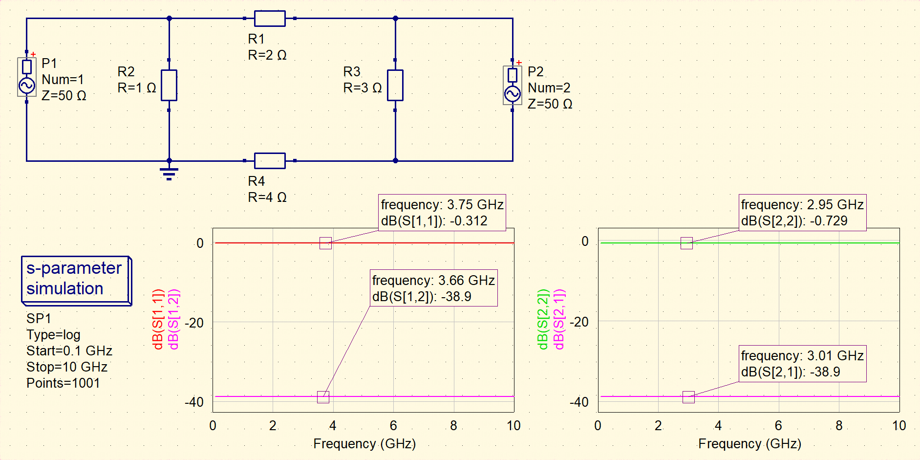Fig.10 Qucs simulation of square-network

4.2 Isolated TSV equivalent circuit model⁵

Let us go a little bit further. We consider an isolated TSV structure with a simple equivalent circuit model in Ref. [5].

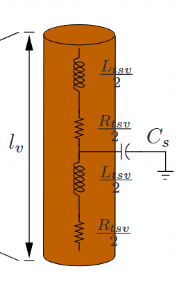Fig.11 circuit model of isolated TSV

As we can see in the Figure, it is a typical T-network. In order to further validate the theory and code, we can provide some value for the parasite parameter.

In the python, we can use the following to simulate the TSV circuit model,

class IsolatedTSV():
    """ 
    Isolated TSV model in Weerasekera2009.
    """
    def __init__(self, L, C, R, Z0, f_low, f_high, N):
        """
        Initializes the TSV parameters.
        """
        self.L = L
        self.C = C
        self.R = R
        self.Z0 = Z0
        self.f_low = f_low
        self.f_high = f_high
        self.N = N
        self.f = np.logspace(np.log10(f_low), np.log10(f_high), N)
        self.w = 2 * np.pi * self.f

        self.Z = np.zeros(shape=(2, 2, N), dtype=np.complex128)
        self.S = np.zeros(shape=(2, 2, N), dtype=np.complex128)

        self.za = self.R / 2.0 + 1j * self.w * self.L / 2.0
        self.zb = self.za
        self.zc = 1. / (1j * self.w * self.C)

        for i in range(N):
            
            isolated_tsv = TNetwork(self.za[i],
                                    self.zb[i],
                                    self.zc[i] , 50)
            
            self.S[:, :, i] = isolated_tsv.S
            self.Z[:, :, i] = isolated_tsv.Z
            
isotsv = IsolatedTSV(L_tsv, C_tsv, R_tsv, 50, 1e3, 10e9, 1000)

plt.plot(isotsv.f, 20 * np.log10(np.abs(isotsv.S[0, 1, :])), label='Insertion loss')
plt.xscale('log')  
plt.xlabel('Frequency (Hz)')
plt.ylabel('Insertion loss (dB)')
plt.title('Insertion Loss of Isolated TSV')
plt.grid(True)

print("Insertion loss at 10GHz:")
print(20 * np.log10(np.abs(isotsv.S[0, 1, -1])))


### Insertion loss at 10GHz:
### -0.009752507454361247

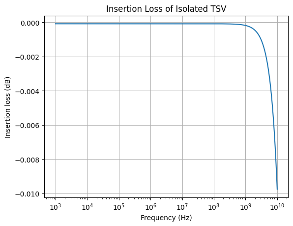Fig.12 Insertion loss of TSV

We can build the circuit model in Qucs Studio as follows,

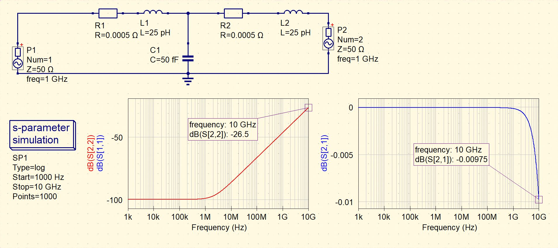Fig.13 Qucs Simulation of circuit model of TSV

As we can see, the simulation of Qucs can successfully validate the results from python code.

5. Conclusion

We have formulate the impedance and scattering matrix of three different structures of networks. The theory is validated by using free software Qucs. To simulate more complicated structure of circuit model, it is encouraged to use cascade theory to build much complicated from these three simple network.

Reference